PowerPivot, Apples and Bananas

Reposted from Thomas Ivarsson blog with the author's permission.

More than 15 years ago I started my professional career in IT as an Excel teacher. One excercise that I frequently used was a simple math problem that you start with in your first year of school as a kid. Make sums of fruits in order to demonstrate how cell references works. I would like to use the same simple example in order to demonstrate how a simple data model in PowerPivot can be built for non database professional and other interested in an introduction to PowerPivot. The model that I will describe is a data model called a starschema.

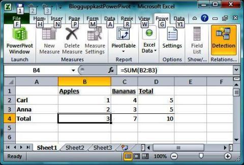
First: Build a simple table in Excel. I use Excel 2010 which is a requirement for the PowerPivot add in for Excel.

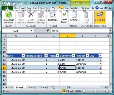
With the word snapshot I describe the table as a state at the end of the day describing what two people(Carl and Anna) have bought from the grocery store. I assume that both have not consumed the fruit yet. The transactions behind this snapshot are the following(see the second picture below). A transactional way of looking at the data is transformed into a summary about the state at the end of  a day regarding how many fruits that Carl and Anna have bought.

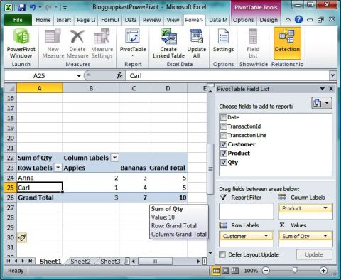
The table above is formatted by using the Format as Table button in the Excel ribbon. On top of the transaction table above you can create a Pivot Table by using place the cursor in the transaction table and select Insert and Pivot Table in the Ribbon. The result is seen in the next picture below. This is how most end users use their table shaped data and Pivot Tables in their daily work.

The example above is not how PowerPivot will work in the best way but a current praxis by many Excel users. PowerPivot will require you to organize the data differently than the data dumps in a spreadsheet. Remember that for this simple example PowerPivot is not necessary but I like to use simple examples to demonstrate a more complex scenario of how you can organize data in the best way. That is also the structure of the data that will be presented to Excel end users.

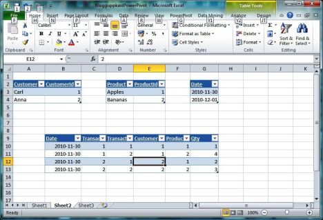
I have constructed four small tables in the same Excel sheet above.  Three of the tables are dimension tables(Customer, Product and Date) and in the real world they will have more columns than in this simple model. The table with most columns, below the dimension tables, is the fact table that contains one measure(Qty) and the other columns are connectors to each dimension table above. Be aware of that I have called the customer identifier in the dimension table CustomerId but Customer in the fact table. When I add these surrogate keys, like they are called technically, the customer can change name. The surrogate key will be the same.  I have the same setup with the product dimension and the fact table.

Why would you do something complex like this when it is possible to do this much more simple, like the examples that I showed earlier? If you think a little bigger and imagine that you will have dimension tables with thousands of products and customers and maybe 1-2 million rows in the fact table. Also you will probably get these tables from the source system that are structured like the mini tables that I show in this spreadsheet. You can simply enter the same data and then format each mini table as a table by the format as table option in Excel.

In the next step will will add each table above to a PowerPivot model by using Linked Tables in PowerPivot.

Place the cursor in each mini table in the Excel spreadsheet and select the “Create Linked Table” under PowerPivot in the Excel ribbon.

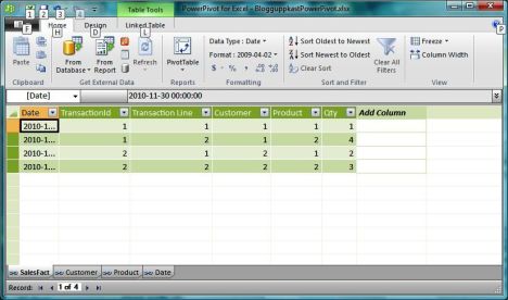
After you have imported these tables you can see them in the PowerPivot window as separate tabs. I have renamed the tables with more descriptive names than table1.

Relations are defined from the fact table to the dimension tables in PowerPivot.

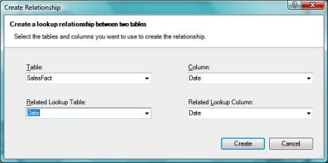
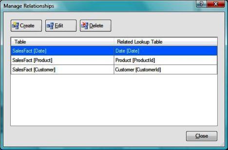
I have defined a relation between the date column in the sales fact column and the Date column in the Date table. In the last step we will have to define the relations between the tables that we have added to the PowerPivot model.  Under the design tab in the PowerPivot Table Tool you can see the Manage Relationships button to get the dialoge window below.

After all relations between the dimension tables and the fact table have been defined you will see the following relations.

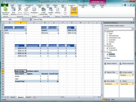
Below is the final report build in Pivot Tables with the PowerPivot tables as the data source. I also show the start micro tables in the spreadsheet but the data in them has been copied in to the PowerPivot data store.

---

Thomas Ivarsson has been working with the MS BI platform since SQL Server 7 in 1999. Presently he is working in the telecom industry in Sweden, with a data warehouse based on SQL Server 2005. From 1999 to 2007 he worked as a consultant also on the three SQL Server BI platforms. During the latest years he has spent most of time on SSAS, Reporting Services, ProClarity and Performance Point. He also has several years experience of the ETL process with DTS and SSIS. During 2008 and 2009 he has been working with introducing data mining in his daily business to see patterns in a service network behaviours. His blog can be found here: http://thomasivarssonmalmo.wordpress.com/

---